Optimizers, Gradient Descent & How neural networks can learn

2026-01-08

I’ve recently gained an interest in how neural networks actually learn, and have been studying the math behind loss landscapes, gradient descent and convexity. Though there are sections in this article, every topic is quite interconnected with one another

Loss Landscapes

Before we dive into gradient descent, there are a few precursors and terms we must become acquainted with.

Later, when we talk about a function $f$, we mean the function that maps our loss, this function creates a loss landscape, in which gradient descent must traverse

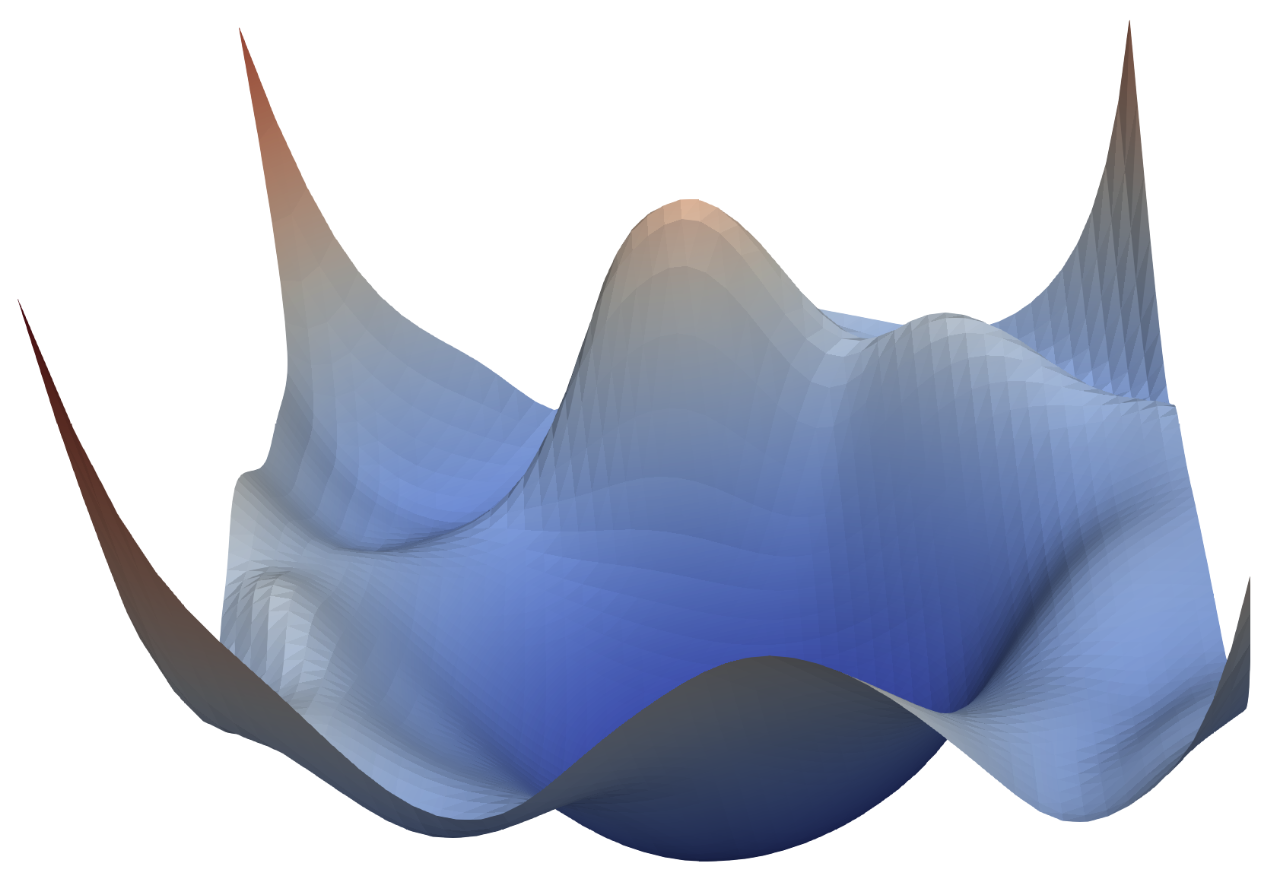
A loss landscape is a high dimensional plane, often visualized 3 dimensions with the x and y axes being directions in parameter space and the z axis being the loss at that point. And so every point in this landscape represents the loss attained when using those parameters.

Our goal is to find local minima, points where the loss is close to the lowest.

Why not the global minimum?

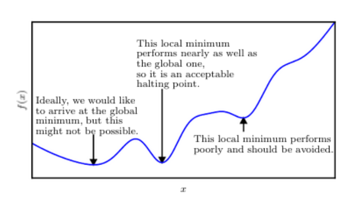
This image from the deep learning book describes it quite well, even though a global minimum does indeed exist, there is little point to optimizing further than a local minima that is “good enough” for the job.

Convex and Non-Convex Functions

Non-Convexity

Earlier, when we talked about loss landscapes and our function $f$, I provided an image of a loss landscape, with all of its bumps, hills, saddle points and rough terrain, what I have explained is the most common function in deep learning, which is a non-convex function.

Convexity

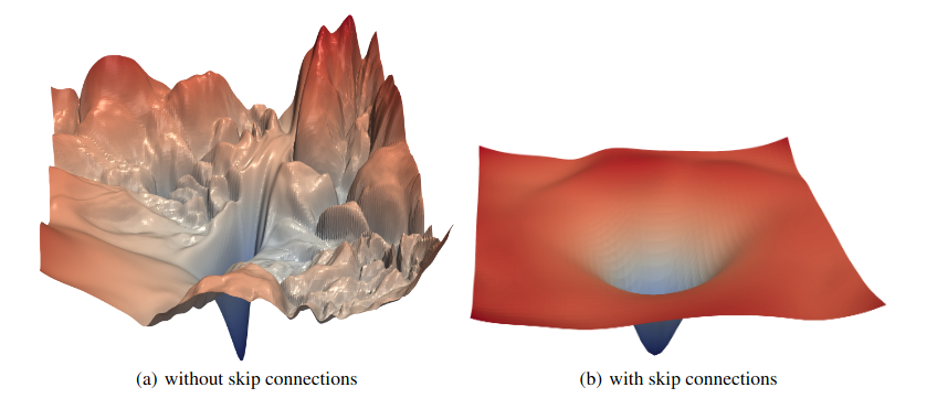
A convex function can be describe as a bowl, any local minima you encounter, is a global minimum, any direction of descent leads right down to the global minimum, as bowls don’t have any bumps in them luckily. By having a convex function, gradient descent becomes much easier, no matter what, it will converge to the global minimum, you can easily prove convergence rates, and you can do learning rate analysis.

And you may ask, if convex functions are so much better, why are they so hard to get? It’s because, neural networks in themselves are non-convex. The composition of linear layers with non-linear activation functions create non-convex optimization landscapes in multi-layer networks.

Gradient Descent

Behind every model, there is a simple algorithm made all the way back in 1847, the gradient descent optimization, at its core, when updating model parameters $\theta$ on function $f$, we take a step in the gradient

with $\alpha$ representing the learning rate

Gradient descent is also a first-order optimization algorithm, meaning we only use the first derivative, and it only knows about its current position in the parameter space, $\theta$ and slope, $\nabla f(\theta)$

Something interesting about gradient descent can be shown to converge to a critical point given:

• A function $f$ that maps the loss landscape, must be continuously differentiable
• The step size is small enough (We’ll touch on this more later)
• $f$ is bounded below (doesn’t go to $-\infty$)

So how does gradient descent work? Given all that it has to traverse, and the fact that its first-order, gradient descent still does shockingly well.

This exact question is still a very active research question, a good argument is that the local minima are quite good, I’m sure that any LLM you may use isn’t the most optimal it can ever be, even they are still using local minima. Overparameterized models appear to avoid poor local minima

Learning Rate $\alpha$

Earlier I mentioned that for gradient descent to converge, we need a step size that is small enough, just so we don’t overshoot local minima.

And so if our learning rate is too large, we run the risk of missing local minima completely, by moving in such large steps, but at the same time, a learning rate too small can make the convergence rate take much longer than necessary.

To further study learning rate and models, throughout the rest of this writing, we will restrict our attention a convex quadratic, which serves as a local model of the loss:

Where $A$ is a model of curvature

Theoretically, when given $f$, we can find a learning rate bound, which can balance curvature directions

Where $L = \parallel \nabla^{2}f(\theta) \parallel_{2}$, the largest eigenvalue in the Hessian

This bound ensures stability, but it does not address the differences in curvature across directions

In order to balance convergence rates across eigenvectors for the convex quadratic requires the optimal learning rate:

This formula is beautiful in its simplicity, with $\alpha^{*}$, the convergence rates of $\lambda_{min}$ and $\lambda_{max}$ is balanced.

Unfortunately, this formula requires both the smallest and largest eigenvalues, and the only way to get that is through the Hessian matrix.

Models of Curvature and the Hessian Matrix

A model of curvature tells you how fast the loss is changing as we move through parameter space, it describes how the gradient itself changes through the loss landscape.

Most commonly in theoretical deep learning, we model curvature with the Hessian, at its simplest, the Hessian matrix is a matrix of second derivatives that describe local curvature, so the curvature that’s around a given point:

You can see how the Hessian would be a very beneficial model of curvature, it seems very useful to know what the curvature around us right now is like, it would leave less of the guessing up to gradient descent,

The major issue with the Hessian is its size, given a model of $n$ parameters, the Hessian matrix is therefore $n \times n$ in size, meaning the Hessian scales as $O(n^{2})$, making it computationally infeasible for use in modern models, a more concrete example to think about a relatively small parameter sized model of 1 million. Even with a small model, computing the Hessian, assuming values are stored in float32, would take up 4TB of space.

The Hessian matrix, is a symmetric model of curvature, making it easier to study, and therefore perform eigenvalue decomposition, where

Where $Q$ represents a matrix of eigenvectors, $Q = [q_{1},\dotsc ,q_{n}]$ These are the properties of the Hessian, eigenvalues From the smallest, $\lambda_{1}$ to the largest, $\lambda{n}$. Under stable learning rates, the eigenvectors with the largest eigenvalues converge the fastest, which is why when we start training model, initially there is a huge jump in model accuracy and performance.

Though we are given this simple optimal learning rate, what we do in practice is much different, almost all of the learning rates we use in actual application are achieved from pure experimentation, trial and error.

Why do the largest eigenvalues converge faster?

A larger eigenvalue means that there is steep curvature, the gradient is large, which pulls gradient descent towards it, therefore converging. Whereas smaller eigenvalues take many more iterations or steps,

At each step in gradient descent, the distance between our point and the optimal decreases (hopefully!), we can decompose this optimization process into independent pieces, where we can study each eigenvector and therefore an eigenvalue. We call this the contraction factor

Where: $\lambda_{i}$ is a eigenvalue we want to study $k$ is the number of iterations, or steps $\alpha$ the learning rate

The contraction factor tells us how much the error shrinks per step

Suppose we have $\lambda_{i} = 100$

Suppose that we take 5 steps with gradient descent, $k=5$

This essentially tells us that we are 3% away from the optimal point, which is very good progress for only 5 steps, we’ve pretty much completed convergence.

Meanwhile, a smaller eigenvalue of $\lambda=0.01$

Even if we take 10,000 steps in this situation:

Still, we’re 60% away from the optimal, meaning we have a long way to go to get close to a local minima

Now we can fully appreciate the optimal learning rate equation from earlier, where $\alpha^{*}$ would make both of these eigenvalues converge at the same rate.

And this is exactly why training models feels like diminishing returns, smaller eigenvalues take longer to converge. This gap between theoretical optimality and computational reality is exactly what modern optimizers are trying to bridge.

Modern Optimizers

I’ll be talking about the most popular optimizer to this day, ADAM, though at the moment there is a lot of talk about optimizers such as Muon, Sophia, RMSProp and so fourth.

ADAM (ADAptive Momentum) deals with the eigenvalue convergence problem with approximation. If we can’t compute the Hessian and therefore get the eigenvalues, Adam rescales updates using running statistics of gradient magnitudes, which improves conditioning without having to explicitly model curvature.

Adam tracks two things for each parameter:

1. $m_{t}$ Momentum, which is the exponential moving average of gradients
2. $v_{t}$ An adaptive learning rate, the exponential moving average of the squared gradients

The update rule of gradient descent then becomes

Where $\delta$ is a numerical stability constant, which prevents this update equating to 0.

The most important part here is the $\frac{1}{\sqrt{v_{t}}}$ term. This approximates preconditioning by the inverse square root of the diagonal Hessian, this essentially gives each parameter its own effective learning rate based on the historical gradient variance. This connects directly back to our eigenvalue convergence problem, instead of computing the full Hessian to find $\lambda_{\min}$ and $\lambda_{\max}$, Adam uses $v_t$ to estimate curvature for each parameter.

In practice, this means that in directions where gradients are consistently large (high curvature, large eigenvalues), $\sqrt{v_{t}}$ grows large, so we divide by a larger number, resulting in a smaller step size. Conversely, in flatter directions (small eigenvalues), we take larger steps. This adaptively addresses the eigenvalue imbalance we spent the previous section analyzing.

If you want to see more about what the Adam optimizer does, I highly recommend the original paper

While we can analyze learning rates, curvature, and optimizers in theory, the behavior of deep neural networks remains only partially understood. Practical training still relies on heuristics, intuition, and experimentation.

Image Credits

The Deep Learning Book

arXiv:1712.09913